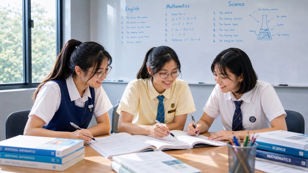
Additional Mathematics Classroom | Chapter 11: Further Applications of Differentiation — Increasing/Decreasing Functions, Stationary Points, First/Second Derivative Tests and Optimisation | SEC G2 K232 / G3 K341

The 2027 SEC position

Both G2 K232 and G3 K341 explicitly require:

• increasing and decreasing functions;
• stationary points, including maximum and minimum turning points and stationary points of inflexion;
• use of the second derivative test to discriminate between maxima and minima;
• application of differentiation to maxima and minima problems.

These requirements sit on top of the shared differentiation engine built in Chapter 10: rational-power differentiation, Product Rule, Quotient Rule and Chain Rule. G3 later extends the function families that can be differentiated, but the logic of increasing/decreasing behaviour, stationary-point classification and optimisation is shared.

Official references: SEAB 2027 G2 Additional Mathematics K232 · SEAB 2027 G3 Additional Mathematics K341.

Finding dy/dx is the beginning. Using its sign, zeros and rate of change is where calculus starts describing behaviour.

---

What this chapter is really teaching

There are two broad jobs.

1. Analyse a given function. Where is it increasing? Where is it decreasing? Where is it stationary? What kind of stationary point occurs?
2. Build and optimise a model. Convert a situation into a one-variable function, differentiate it, locate candidates, classify them and interpret the answer back in the original context.

The first job begins with calculus. The second often begins before calculus. In a maximum-area or minimum-cost problem, the difficult part may be choosing variables and constructing the function. Differentiation can only optimise the function you actually built.

That leads to the governing optimisation loop:

Define → constrain → construct → differentiate → find candidates → classify → compare boundaries → interpret → verify.

Chapter map

1. Higher derivatives and what they mean
2. Increasing and decreasing functions
3. Derivative sign charts
4. Stationary points
5. Turning points versus stationary inflexion
6. First Derivative Test
7. Second Derivative Test
8. When the second derivative test is inconclusive
9. Sketching curves from derivative evidence
10. Minimum and maximum gradient
11. Optimisation architecture
12. Geometric optimisation
13. Area, volume and surface-area problems
14. Algebraic constraint problems
15. Boundary and domain checks
16. Global versus local extrema
17. Verification and numerical checks
18. Common optimisation errors
19. Original guided practice
20. Worked answers and mastery checkpoint

---

1 · Higher derivatives: how the gradient itself is changing

If y = f(x), the first derivative f′(x) describes the gradient of the original function. Differentiate again and we obtain the second derivative f″(x):

f″(x) = d/dx[f′(x)] = d²y/dx².

The second derivative describes how the gradient is changing.

• f″(x) > 0: gradient is increasing locally.
• f″(x) < 0: gradient is decreasing locally.
• f″(x) = 0: the second derivative test may be inconclusive and further analysis can be required.

Worked route

For y = 2x³ − 9x² + 5x + 3:

dy/dx = 6x² − 18x + 5.

d²y/dx² = 12x − 18.

The first derivative is a quadratic gradient function. The second derivative tells us where that gradient function is rising or falling.

Third derivatives and beyond

Higher derivatives can continue, but SEC optimisation and stationary-point work centres mainly on the first and second derivatives. The third derivative may occasionally help understand an inconclusive stationary point, but the first-derivative sign test remains the most direct shared-school method when f″(a) = 0.

---

2 · Increasing and decreasing functions

A differentiable function is increasing on an interval where

f′(x) > 0

and decreasing where

f′(x) < 0.

This makes intuitive sense. A positive tangent gradient points upward as x increases. A negative tangent gradient points downward.

Worked route A · cubic behaviour

Find the intervals on which

f(x) = x³ − 3x² − 9x + 5

is increasing or decreasing.

Differentiate:

f′(x) = 3x² − 6x − 9

= 3(x² − 2x − 3)

= 3(x − 3)(x + 1).

The critical values are x = −1 and x = 3. They split the real line into three intervals.

• x < −1: both factors negative, product positive → increasing.
• −1 < x < 3: one factor negative, one positive → decreasing.
• x > 3: both factors positive → increasing.

Therefore f is increasing for x < −1 and x > 3, and decreasing for −1 < x < 3.

A sign chart is a behaviour map

Instead of substituting many values into the original function, analyse the sign of f′(x). The derivative has compressed the question “how does the curve behave?” into a sign problem.

---

3 · Stationary points: horizontal tangent, not automatically a turning point

A stationary point occurs where

f′(x) = 0.

The tangent is horizontal at that x-value. But the curve does not necessarily turn.

• Maximum turning point: increasing before, decreasing after.
• Minimum turning point: decreasing before, increasing after.
• Stationary point of inflexion: tangent horizontal but the sign of f′(x) does not switch from + to − or − to +; the curve continues through while changing its manner of bending.

This distinction is central. “Set f′(x) = 0” finds stationary candidates. It does not classify them.

Worked route · stationary coordinates

Find the stationary points of

y = x³ − 3x + 2.

dy/dx = 3x² − 3 = 3(x − 1)(x + 1).

Stationary when dy/dx = 0:

x = −1 or x = 1.

At x = −1:

y = −1 + 3 + 2 = 4.

At x = 1:

y = 1 − 3 + 2 = 0.

Stationary points: (−1,4) and (1,0).

Classification comes next.

---

4 · First Derivative Test: classify by sign change

The First Derivative Test asks what happens to the sign of f′(x) as x passes through the stationary value.

• f′ changes + to − → local maximum.
• f′ changes − to + → local minimum.
• f′ stays + on both sides or − on both sides → stationary point of inflexion.

This test is especially valuable because it directly reads the behaviour of the original function.

Classify y = x³ − 3x + 2

f′(x) = 3(x − 1)(x + 1).

For x < −1, f′ > 0.

For −1 < x < 1, f′ < 0.

For x > 1, f′ > 0.

At x = −1, sign changes + → −, so (−1,4) is a maximum turning point.

At x = 1, sign changes − → +, so (1,0) is a minimum turning point.

Stationary inflexion example

Consider y = x³ − 1.

dy/dx = 3x².

Stationary at x = 0, point (0,−1).

For x < 0, 3x² > 0. For x > 0, 3x² > 0.

The function is increasing on both sides. Therefore (0,−1) is a stationary point of inflexion, not a maximum or minimum.

---

5 · Second Derivative Test: classify by how the gradient is changing

At a stationary point x = a where f′(a) = 0:

• if f″(a) < 0, the gradient is decreasing through zero → local maximum;
• if f″(a) > 0, the gradient is increasing through zero → local minimum;
• if f″(a) = 0, the test is inconclusive.

Worked route

Find and classify the stationary points of

y = 2x³ + 3x² − 12x + 7.

dy/dx = 6x² + 6x − 12

= 6(x + 2)(x − 1).

Stationary at x = −2 and x = 1.

At x = −2:

y = 2(−8)+3(4)+24+7 = 27.

At x = 1:

y = 2+3−12+7 = 0.

Second derivative:

d²y/dx² = 12x + 6.

At x = −2:

f″(−2) = −18 < 0 → maximum at (−2,27).

At x = 1:

f″(1) = 18 > 0 → minimum at (1,0).

Why the test works

At a maximum, the gradient typically moves from positive to zero to negative. The gradient is decreasing through the stationary point, so f″ is negative. At a minimum, the gradient moves from negative to zero to positive, so f″ is positive.

---

6 · When f″(a) = 0: inconclusive does not mean inflexion

If the second derivative at a stationary point is zero, do not automatically call it a stationary point of inflexion. The Second Derivative Test has simply failed to classify the point.

Return to the First Derivative Test and inspect the sign of f′ on either side.

Example A · stationary inflexion

y = x³.

y′ = 3x², so stationary at x = 0.

y″ = 6x, so y″(0) = 0.

But y′ is positive on both sides, so the point is a stationary inflexion.

Example B · minimum even though f″ = 0

y = x⁴.

y′ = 4x³, so stationary at x = 0.

y″ = 12x², so y″(0) = 0.

Yet y′ is negative for x < 0 and positive for x > 0. Therefore the origin is a minimum.

This counterexample is essential. Zero second derivative does not identify the stationary-point type.

---

7 · Sketching a curve from derivative evidence

A complete sketch uses several kinds of evidence:

• intercepts where easy to find;
• stationary-point coordinates;
• classification of those points;
• increasing/decreasing intervals;
• end behaviour from the leading term;
• symmetry or factorisation when available.

Worked sketch architecture

For y = x³ − 3x + 2:

• stationary maximum at (−1,4);
• stationary minimum at (1,0);
• y-intercept (0,2);
• factorisation y = (x − 1)²(x + 2), so x-intercepts at x = −2 and x = 1, with x = 1 a repeated root;
• leading term x³ → graph goes down to the left and up to the right.

The derivative tells us the shape between key points; factorisation tells us how the curve meets the x-axis.

Repeated roots and stationary contact

At x = 1, the repeated factor (x − 1)² means the graph touches the x-axis rather than crossing. The derivative also vanishes there. Algebra and calculus are describing the same geometry from different directions.

---

8 · Minimum or maximum gradient: optimise the derivative itself

The old textbook includes an elegant extension: sometimes the quantity to minimise is not y but the gradient dy/dx.

If z = dy/dx, then finding a minimum gradient means optimising z as a function of x.

Differentiate z:

dz/dx = d²y/dx².

Set dz/dx = 0 to find stationary values of the gradient function.

Worked route · minimum gradient

Find the minimum gradient of

y = 2x³ − 9x² + 5x + 3

and the x-value at which it occurs.

Gradient function:

z = dy/dx = 6x² − 18x + 5.

Differentiate z:

dz/dx = 12x − 18.

Stationary gradient when:

12x − 18 = 0 → x = 3/2.

z(3/2) = 6(9/4) − 18(3/2) + 5

= 13.5 − 27 + 5

= −8.5.

Since z is an upward-opening quadratic—or because its second derivative is positive—the stationary value is a minimum.

Thus the minimum gradient is −8.5 at x = 1.5.

This problem makes the derivative hierarchy visible: y describes the curve; y′ describes its gradient; y″ helps locate extreme values of that gradient.

---

9 · Optimisation begins before differentiation

In a word problem, do not begin by differentiating whatever expression appears first. First identify:

1. Objective: what quantity is being maximised or minimised?
2. Constraint: what relationship limits the variables?
3. Independent variable: which variable will remain free?
4. Domain: what values are physically or mathematically possible?

Use the constraint to eliminate extra variables until the objective is expressed as a one-variable function. Only then differentiate.

The optimisation template

Objective Q = … → use constraint → Q(x) → Q′(x)=0 → classify → check domain/boundaries → return to context.

Why one variable matters

If area A = xy and both x and y are still free, dA/dx is not enough unless y has been expressed in terms of x or another calculus framework is being used. SEC single-variable optimisation expects the constraint to reduce the problem first.

---

10 · Geometric optimisation: a rectangle beside a river

A farmer has 600 m of fencing to enclose a rectangular pen beside a straight river. The river forms one side, so only three sides need fencing. Find the dimensions that maximise area.

Let x be the width perpendicular to the river and y the fenced side parallel to the river.

Constraint:

2x + y = 600.

So y = 600 − 2x.

Objective area:

A = xy

= x(600 − 2x)

= 600x − 2x².

Domain: 0 < x < 300.

Differentiate:

dA/dx = 600 − 4x.

Set zero:

600 − 4x = 0 → x = 150.

Then y = 600 − 300 = 300.

Second derivative:

d²A/dx² = −4 < 0, so this is a maximum.

Therefore the maximum-area dimensions are 150 m by 300 m, with the 300 m side parallel to the river.

The calculus was one line. The modelling—choosing x, using the three-side fencing constraint and building A(x)—was the real setup.

---

11 · Closed cylinder with fixed surface area: minimise or maximise what remains

A classic optimisation structure uses a right circular cylinder with radius r and height h.

• Volume V = πr²h.
• Closed surface area S = 2πr² + 2πrh.

If S is fixed, the constraint allows h to be written in terms of r:

2πr² + 2πrh = S.

Divide by 2πr:

r + h = S/(2πr).

Hence

h = S/(2πr) − r.

Substitute into V:

V(r) = πr²[S/(2πr) − r]

= Sr/2 − πr³.

Then

dV/dr = S/2 − 3πr².

The stationary condition gives

r² = S/(6π).

The second derivative −6πr is negative for r > 0, so the stationary value is a maximum.

The important learning point is not the final formula. It is the sequence: surface-area constraint → eliminate h → build V(r) → differentiate.

Dimensional check

S/(6π) has units of area, so r² has units of area. That is dimensionally sensible. Unit checking is a quiet way to catch modelling algebra errors.

---

12 · Constraint optimisation without geometry

Optimisation may involve algebraic relationships rather than a diagram.

Worked route · x + y = 5

Given x + y = 5, find the maximum value of

Q = 2x² + xy − 3y².

Use y = 5 − x.

Q(x) = 2x² + x(5 − x) − 3(5 − x)².

Expand:

Q = 2x² + 5x − x² − 3(25 − 10x + x²)

= x² + 5x − 75 + 30x − 3x²

= −2x² + 35x − 75.

Differentiate:

Q′ = −4x + 35.

Stationary when x = 35/4.

Then y = 5 − 35/4 = −15/4.

Q″ = −4 < 0, so this is a maximum over the unrestricted real constraint line.

The example shows why context matters. If x and y represented positive lengths, this stationary point would violate y > 0 and could not be accepted. A purely algebraic constraint and a physical constraint may have different admissible domains.

---

13 · Boundary checks: a stationary point may not be the global optimum

The equation Q′(x) = 0 finds interior stationary candidates. A global maximum or minimum on a restricted interval may also occur at an endpoint.

For example, suppose a function is to be minimised for 0 ≤ x ≤ 4. If its only stationary point lies at x = 2, compare f(0), f(2) and f(4) before claiming the global minimum.

In physical optimisation, endpoints often correspond to degenerate shapes—zero height, zero width or exhausted resources. Even when those endpoints are excluded, understanding their limiting behaviour helps confirm that the interior stationary point is the relevant optimum.

Local versus global

• Local maximum: larger than nearby values.
• Global maximum: largest value over the entire stated domain.
• Local minimum: smaller than nearby values.
• Global minimum: smallest value over the entire stated domain.

The second derivative classifies local behaviour. Domain and boundary comparison are what justify a global claim.

---

14 · Optimisation with a square sheet: modelling before calculus

A square sheet of side 20 cm has equal squares of side x cut from each corner. The sides are folded to form an open box. Find the x that maximises volume.

After cutting:

• height = x;
• length = 20 − 2x;
• width = 20 − 2x.

Domain:

0 < x < 10.

Volume:

V = x(20 − 2x)².

One efficient derivative route keeps the product structure:

V′ = (20 − 2x)² + x·2(20 − 2x)(−2).

Factor:

V′ = (20 − 2x)[(20 − 2x) − 4x]

= (20 − 2x)(20 − 6x).

Stationary candidates:

x = 10 or x = 10/3.

x = 10 is the boundary where the base collapses and volume is zero. The interior candidate is x = 10/3.

Since the volume is zero near the degenerate boundaries and positive inside, or by derivative sign/second derivative classification, the maximum occurs at

x = 10/3 cm.

The factor x = 10 emerged from the algebra but is not an interior physical stationary box. Domain interpretation filters the mathematics.

---

15 · Maximum/minimum problems are often hidden quadratics or cubics

Some optimisation problems reduce to a quadratic, which could also be solved by completing the square. Others become cubic or rational functions where differentiation is the natural tool.

When a quadratic objective appears, using calculus still has value because it connects the result to the broader optimisation method. But alternative methods are excellent verification.

Two-method check

For A(x) = 600x − 2x²:

calculus gives A′ = 600 − 4x = 0 → x = 150.

Completing the square gives

A = −2(x² − 300x)

= −2[(x − 150)² − 22500]

= −2(x − 150)² + 45000.

The same maximum x-value and maximum area appear. Independent agreement increases confidence.

---

16 · Verification: optimisation answers deserve more than one check

• Derivative check: does Q′(x*) = 0?
• Classification check: does the first/second derivative support maximum or minimum?
• Domain check: is x* physically/mathematically admissible?
• Boundary check: could an endpoint beat the stationary value?
• Units check: does the final quantity have the correct units?
• Model check: do all derived dimensions or variables remain possible?
• Alternative-method check: for a quadratic, does completing the square agree?
• Numerical-neighbour check: do nearby values behave as expected around the claimed optimum?

Neighbour check

If x* is claimed to maximise a function, evaluate the function at x* − small amount and x* + small amount where sensible. Both should be slightly lower for a smooth local maximum. This is not a proof, but it is an effective error detector.

---

17 · Common stationary-point and optimisation errors

• Stationary = maximum error: setting f′ = 0 and declaring “maximum” without classification.
• Second derivative zero misclassification: treating f″ = 0 as proof of stationary inflexion.
• Coordinate omission: finding stationary x-values but not returning to f(x) for y-coordinates.
• Sign-chart omission: failing to identify increasing/decreasing intervals when requested.
• Objective confusion: differentiating the constraint instead of constructing the quantity to optimise.
• Too-many-variables error: differentiating A = xy before eliminating y with the constraint.
• Domain omission: accepting negative lengths or degenerate dimensions.
• Boundary omission: claiming global maximum/minimum from one interior stationary point without checking the stated interval.
• Wrong quantity returned: finding x but the question asks for maximum volume, dimensions or cost.
• Unit omission: giving “45000” instead of an area with square units.
• Rounding too early: approximating a stationary value before substituting into the objective.
• Minimum-gradient confusion: optimising y instead of y′.

The first weak-link test

1. Can the learner find f′?
2. Can the learner solve f′ = 0?
3. Can the learner find stationary coordinates?
4. Can the learner classify using first or second derivative?
5. Can the learner identify increasing/decreasing intervals?
6. Can the learner turn a word problem into one objective function?
7. Can the learner enforce the domain?
8. Can the learner return the answer requested by the context?

---

18 · G2 and G3: shared optimisation logic

The calculus logic in this chapter is shared across G2 and G3. Both levels must analyse derivative signs, stationary points, second derivative classification and maximum/minimum applications.

• G2: stabilise the analysis loop on algebraic functions and clearly structured contexts.
• G3: use the same loop on a wider range of functions, including later trigonometric, exponential and logarithmic derivatives, and in denser mixed-topic settings.

The optimisation method does not change when the function family changes. The derivative engine becomes broader; the reasoning architecture stays the same.

---

19 · Original guided practice

The questions below are original to this classroom guide. They progress from sign analysis and stationary points into full contextual optimisation.

A · Increasing and decreasing functions

1. Find the intervals where f(x) = x³ − 3x² − 9x + 5 is increasing and decreasing.
2. Find the intervals where f(x) = 2x³ + 3x² − 12x + 7 is increasing and decreasing.
3. Find the values of x for which f(x) = x⁴ − 4x² is decreasing.
4. Given f′(x) = (x − 2)²(x + 1), determine the intervals where f is increasing or decreasing.
5. Given f′(x) = −(x + 3)(x − 1), determine the behaviour intervals.

B · Stationary points and classification

6. Find and classify the stationary points of y = x³ − 3x + 2.
7. Find and classify the stationary points of y = 2x³ + 3x² − 12x + 7.
8. Find and classify the stationary points of y = x⁴.
9. Find the stationary point of y = x³ − 1 and determine its nature.
10. Find and classify all stationary points of y = x⁴ − 2x³.
11. Find the stationary points of y = (x + 2)(x − 1)² and determine their nature.

C · First versus second derivative tests

12. Explain why f″(a) < 0 at a stationary point implies a local maximum.
13. Explain why f″(a) = 0 is inconclusive.
14. Give one function with f′(0)=0 and f″(0)=0 where x=0 is a minimum.
15. Give one function with f′(0)=0 and f″(0)=0 where x=0 is a stationary point of inflexion.
16. For f′(x) = (x − 1)²(x + 2), classify the stationary values x = 1 and x = −2 using sign changes.

D · Minimum and maximum gradient

17. Find the minimum gradient of y = 2x³ − 9x² + 5x + 3.
18. Find the minimum gradient of y = 5x³ − 24x² + 7x − 5 and the x-value where it occurs.
19. For y = x³ + 6x² − 3x, find the minimum value of dy/dx.
20. Explain why the stationary points of the gradient function are found using d²y/dx² = 0.

E · Geometric optimisation

21. A rectangle beside a river uses 600 m of fencing on three sides. Find the dimensions that maximise area.
22. A rectangle has perimeter 80 cm. Find the side lengths that maximise area.
23. A square sheet of side 20 cm has x-cm squares cut from each corner and is folded into an open box. Find the x that maximises volume.
24. A right triangle has perpendicular sides x and y with x + y = 20. Find the maximum possible area.
25. A rectangle is inscribed under the parabola y = 12 − x² with its base on the x-axis and symmetric about the y-axis. Express its area in terms of x and find the maximum area.

F · Constraint and modelling optimisation

26. Given x + y = 5, find the stationary value of Q = 2x² + xy − 3y² and classify it.
27. Positive numbers x and y satisfy x + y = 18. Find the maximum product xy.
28. Positive numbers x and y satisfy 2x + y = 24. Find the maximum value of xy.
29. A closed cylinder has fixed surface area S. Show that the radius that maximises volume satisfies r² = S/(6π).
30. A closed cylinder has surface area 600π cm². Find the radius that maximises its volume.
31. An open-top square-based box has volume 108 cm³. If its base side is x, express the surface area in terms of x and find the x that minimises surface area.

G · Domain, boundaries and interpretation

32. Why must an optimisation model for a physical length include a domain?
33. A stationary candidate gives x = −3 cm for a side length. What should happen next?
34. A function is optimised on 0 ≤ x ≤ 5 and has a stationary point at x = 2. What values must be compared to establish a global maximum?
35. Explain the difference between local and global maximum.
36. A volume function has stationary values at x = 4 and x = 10, but x = 10 makes one dimension zero. Explain why x = 10 is not the desired physical optimum.

H · Mixed SEC reasoning

37. A student sets f′(x)=0 and immediately writes “maximum”. Diagnose the missing step.
38. A student finds f″(a)=0 and writes “stationary point of inflexion”. Give a counterexample.
39. A student finds the correct x-value for maximum area but never calculates the dimensions requested. Diagnose the answer-form error.
40. A student optimises A = xy while x and y are linked by x + y = 10 but never substitutes the constraint. Explain why the calculus setup is incomplete.
41. A student substitutes x = 4 into the objective before differentiating. Explain why this may destroy the variable relationship.
42. For a quadratic objective, explain how completing the square can verify a calculus maximum/minimum.
43. Why can a factorised derivative be particularly useful in stationary-point analysis?
44. Explain why a sign chart for f′ gives more information than only solving f′ = 0.
45. State the shared G2/G3 optimisation content and the later G3 function-family extension.

20 · Worked answers and reasoning checkpoints

1. f′=3(x−3)(x+1). Increasing x<−1 or x>3; decreasing −1<x<3.
2. f′=6(x+2)(x−1). Increasing x<−2 or x>1; decreasing −2<x<1.
3. f′=4x³−8x=4x(x²−2). Sign analysis gives decreasing on (−∞,−√2)?? Check carefully: choose x=−2 gives f′ negative; x=−1 gives positive; x=1 gives negative; x=2 gives positive. Thus decreasing on (−∞,−√2) and (0,√2).
4. At x=−1 sign changes negative→positive because squared factor at 2 does not change sign; at x=2 sign does not change. Thus increasing/decreasing intervals follow the sign of x+1 except for the zero at 2: decreasing x<−1; increasing x>−1, with stationary inflexion behaviour at x=2 if the underlying function is differentiable.
5. f′=−(x+3)(x−1). Negative outside roots and positive between: decreasing x<−3 and x>1; increasing −3<x<1.
6. (−1,4) maximum; (1,0) minimum.
7. (−2,27) maximum; (1,0) minimum.
8. y′=4x³; stationary x=0. Sign −→+, so (0,0) minimum; second derivative zero there is inconclusive.
9. y′=3x² positive on both sides, so (0,−1) stationary point of inflexion.
10. y′=4x³−6x²=2x²(2x−3). Stationary x=0 and 3/2. At x=0 sign stays negative on both sides → stationary inflexion. At x=3/2 sign changes −→+ → minimum; y(3/2)=81/16−27/4=−27/16.
11. Expand y=(x+2)(x−1)²=x³−3x+2, giving the same stationary points (−1,4) max and (1,0) min.
12. At a stationary point f′=0. If f″<0, f′ is decreasing through zero, so it changes from positive to negative locally, giving a maximum.
13. Because functions such as x⁴ and x³ both have f′(0)=f″(0)=0 but have different stationary behaviour.
14. f(x)=x⁴.
15. f(x)=x³.
16. f′=(x−1)²(x+2). At x=−2 sign changes −→+ → minimum. At x=1 the squared factor does not change sign → stationary inflexion.
17. −8.5 at x=1.5.
18. Gradient z=15x²−48x+7. Minimum occurs at x=48/30=8/5. z(8/5)=15(64/25)−48(8/5)+7=38.4−76.8+7=−31.4, i.e. −157/5.
19. y′=3x²+12x−3=3[(x+2)²−5]. Minimum at x=−2, value −15.
20. Because z=y′ is the quantity being optimised; z′=y″. Stationary values of z occur where y″=0.
21. 150 m by 300 m.
22. Let sides x and 40−x. A=x(40−x)=40x−x². A′=40−2x=0 gives x=20; square 20 cm by 20 cm.
23. V=x(20−2x)²; interior maximum at x=10/3 cm.
24. y=20−x. Area=(1/2)x(20−x)=10x−x²/2. A′=10−x=0, so x=y=10; max area 50.
25. Top corners at (±x,12−x²), so width=2x and height=12−x². A=2x(12−x²)=24x−2x³, with 0<x<√12. A′=24−6x²=0 gives x=2. Area=32 square units.
26. As derived, Q=−2x²+35x−75, stationary x=35/4, y=−15/4, and Q″=−4 so maximum on the unrestricted real constraint.
27. Product P=x(18−x)=18x−x². P′=18−2x=0 gives x=y=9, max product 81.
28. y=24−2x. P=x(24−2x)=24x−2x². P′=24−4x=0 → x=6, y=12. Max 72.
29. As shown: r²=S/(6π).
30. S=600π, so r²=100 and r=10 cm.
31. Volume x²h=108, so h=108/x². Surface area S=x²+4xh=x²+432/x. S′=2x−432/x²=0 gives 2x³=432, x³=216, so x=6 cm. Then h=3 cm. S″=2+864/x³>0, so minimum.
32. Because the algebra may produce values that do not represent possible lengths, times, masses or dimensions. The domain defines admissible candidates.
33. Reject it as a physical side length and continue checking other candidates/boundaries.
34. Compare f(0), f(2), f(5).
35. Local maximum exceeds nearby values; global maximum exceeds all values on the stated domain.
36. x=10 collapses a dimension and produces a degenerate box/shape, typically a boundary with zero volume rather than the desired interior optimum.
37. Classification is missing: use first-derivative sign change or second derivative test, plus domain/boundary checks when a global claim is required.
38. x⁴ has f′(0)=0 and f″(0)=0 but x=0 is a minimum, not an inflexion.
39. The question asks for dimensions, not only the internal stationary variable. Substitute back into the constraint and report the requested quantities with units.
40. The objective still depends on two variables. Use y=10−x first so the objective becomes a one-variable function.
41. Substituting the candidate first freezes the variable and can turn the objective into a constant, removing the dependence that differentiation needs.
42. Complete the quadratic into vertex form. Its explicit maximum/minimum should agree with the derivative result.
43. Factorisation exposes the roots of f′ directly and makes sign changes easier to analyse.
44. Solving f′=0 gives only stationary locations. A sign chart also shows increasing/decreasing intervals and classifies the sign change around stationary points.
45. Both levels require increasing/decreasing functions, stationary points including stationary inflexion, second derivative discrimination, and maxima/minima applications. G3 later applies the same logic to a wider derivative family including trig, exponential and logarithmic functions.

Correction check on Question 3: for f′=4x(x²−2), the sign is negative on (−∞,−√2), positive on (−√2,0), negative on (0,√2), positive on (√2,∞). This is why interval testing matters more than guessing from the factor order.

---

21 · A two-week stationary-point and optimisation architecture

1. Day 1: derivative sign charts and increasing/decreasing intervals.
2. Day 2: stationary coordinates and first derivative classification.
3. Day 4: second derivatives and the inconclusive f″=0 case.
4. Day 6: curve sketches from stationary evidence.
5. Day 8: minimum-gradient problems.
6. Day 10: simple quadratic optimisation with domain.
7. Day 12: geometric and volume optimisation requiring a constraint.
8. Day 14: mixed optimisation with boundary/global checks and unlabelled contexts.

Seven-minute retrieval test

• What does f′>0 mean?
• What does f′<0 mean?
• What defines a stationary point?
• State the three First Derivative Test sign patterns.
• State the Second Derivative Test for maxima/minima.
• What must you do when f″=0?
• State the optimisation loop from objective to interpretation.
• Why must boundaries be checked on a closed interval?

22 · For teachers: separate candidate-finding from classification

A common teaching shortcut is “differentiate, equal zero, maximum/minimum”. Replace it with two explicit questions:

1. Where is the function stationary?
2. What kind of stationary point is it?

Students should feel that classification is a separate mathematical job. This prevents the habitual error of labelling every stationary point as a turning point.

Teach f″=0 with contrasting examples

Put x³ and x⁴ side by side. Both have f′(0)=0 and f″(0)=0. One is stationary inflexion; one is minimum. That single contrast inoculates students against an extremely common false rule.

Optimisation lessons should spend time before the derivative

Ask students to identify the objective, constraint, variable and domain before any calculus is allowed. If the function is built incorrectly, perfect differentiation cannot rescue the model.

23 · For parents: what real progress sounds like

A student relying on procedure may say, “I set the derivative to zero because it says maximum.” A student gaining control begins to say:

• “dy/dx = 0 gives the candidates; I still need to classify them.”
• “The derivative changes from positive to negative, so this is a maximum.”
• “The second derivative is zero, so the test is inconclusive; I need the first derivative sign.”
• “The question asks for maximum volume, so volume is my objective—not surface area.”
• “I need to use the fencing condition to remove y before I differentiate.”
• “This stationary value gives a negative length, so it is outside the physical domain.”
• “Because the interval is closed, I need to compare the endpoints too.”

This language shows the learner is operating the optimisation system rather than treating differentiation as a ritual.

24 · What carries forward

The old textbook’s next chapter is Differentiation of Trigonometric, Logarithmic & Exponential Functions and their Applications. Under SEC 2027 this becomes a clear G3-only extension: K341 requires derivatives of sin x, cos x, tan x, e^x and ln x, while K232 does not list those derivative families.

The next classroom article will therefore keep the calculus application architecture learned here but broaden the objects that can be differentiated. That is a better modern route than mixing the function-family extension into the shared calculus floor and obscuring the G2/G3 boundary.

---

Official syllabus references

• Singapore Examinations and Assessment Board · 2027 SEC G2 Additional Mathematics K232
• Singapore Examinations and Assessment Board · 2027 SEC G3 Additional Mathematics K341

Curriculum and assessment requirements can change. The official SEAB syllabuses remain the controlling sources for current subject codes, examinable content and examination structure.

Return to the Additional Mathematics Learning Hub