
Parents searching for Secondary Mathematics tuition in Sengkang often compare statistics tuition, probability, data handling, averages, graphs, cumulative frequency, sample spaces, combined events and exam preparation. These topics are sometimes treated as separate chapters, but they share a common job: make sensible conclusions from incomplete, variable or uncertain information.
A strong Secondary Math tutor in Sengkang should therefore teach students how to read data, choose appropriate summaries, recognise misleading representations, construct sample spaces and reason about chance. A student who can calculate a mean but cannot explain whether the mean is representative has only part of the skill. A student who can multiply probabilities mechanically but cannot define the event space is equally fragile.
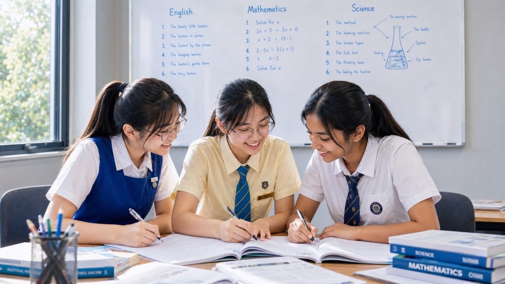
At eduKate Sengkang, statistics and probability are taught in small groups of up to three students. That makes it possible to inspect not only calculations but interpretation. One learner may misread a scale, another may choose the wrong average, and a third may assume events are equally likely when they are not. The first weak link determines the repair.
The One-Sentence Goal
A strong learner can organise data, summarise it appropriately, judge what the summary does and does not show, and model chance events without inventing certainty.
Statistics Is About More Than Calculation
Statistics helps us describe groups, compare patterns and reason from samples. The calculations matter, but interpretation gives them meaning.
If two classes both have an average score of 70, they may still be very different. One class may have most students near 70. Another may have scores spread widely from 40 to 100. A single average hides that difference.
What “Weak in Statistics” Can Actually Mean
| Visible problem | Possible first weak link | What we investigate |
|---|---|---|
| Mean is calculated incorrectly | Total-frequency control | Can the learner distinguish sum of values from number of values? |
| Wrong average chosen | Interpretation | Does the student understand mean, median and mode as different summaries? |
| Graph conclusions are exaggerated | Scale and representation | Can the learner read axes and intervals before interpreting visual size? |
| Frequency tables cause errors | Data organisation | Can the student distinguish value from frequency? |
| Probability answers exceed 1 | Probability scale | Does the learner understand probability as a number between 0 and 1 inclusive? |
| Combined events are guessed | Sample-space structure | Can the learner list outcomes systematically? |
| Multiplication rule is misused | Event relationship | Does the learner know whether events are independent? |
Mean, Median and Mode: Different Questions
The mean uses every value. The median identifies the middle position after ordering. The mode identifies the most frequent value.
Consider the data:
5, 6, 6, 7, 26
The mean is 10, the median is 6 and the mode is 6. The large value 26 pulls the mean upward. If the goal is to describe a typical value, the median may be more representative in this small example.
Students should not ask only “Which formula?” They should ask “What does this summary tell me?”
Range and Spread
Two data sets can share the same mean but have different variability. Range gives a simple first measure:
range = maximum − minimum
As students progress, they may meet more refined measures of spread. The core idea remains: centre alone does not describe distribution fully.
Frequency Tables: Value and Count Are Different
A common error occurs when students add frequencies and values together or forget to multiply each value by its frequency when finding a mean from a frequency table.
If score 4 occurs three times, its contribution to the total is 12. The table compresses repeated observations, so the calculation must reconstruct the total correctly.
Graphs Can Inform or Mislead
Students should read axes, scale and labels before reacting to visual size.
A bar chart whose vertical axis starts at 95 can make values 96 and 99 look dramatically different. The difference is real, but the visual impression may be exaggerated.
We teach students to separate the data from the design of the graph.
Scatter Plots and Association
Scatter plots help students examine relationships between two variables. A general upward pattern suggests positive association; a downward pattern suggests negative association.
But association does not automatically prove causation. If students who sleep more tend to score better, the graph alone does not prove sleep is the only cause. Other factors may influence both variables.
Probability: A Scale of Uncertainty
Probability ranges from 0 to 1.
- 0 means impossible;
- 1 means certain;
- values between represent degrees of chance.
Percentages can also express probability, so 0.25 = 25% = one chance in four under the relevant model.
Sample Space Before Formula
For simple equally likely outcomes:
P(event) = favourable outcomes / total possible outcomes
The formula only works when the outcome space is understood correctly.
If two coins are tossed, the sample space is:
HH, HT, TH, TT
Exactly one head occurs in HT and TH, so the probability is 2/4 = 1/2.
Systematic Listing Prevents Missing Outcomes
Students often lose probability marks because they list outcomes randomly and miss cases. Tables, tree diagrams and ordered pairs make the sample space systematic.
The representation should reduce omission risk.
Independent Events
Two events are independent when the occurrence of one does not change the probability of the other.
For example, rolling a fair die and tossing a fair coin are independent. The probability of rolling a 6 and obtaining a head is:
1/6 × 1/2 = 1/12
The multiplication rule works because the events are independent under the model.
Dependent Events
If a card is drawn from a pack and not replaced, the composition of the pack changes. The probability of the second event now depends on the first.
Students should not multiply probabilities mechanically without checking whether the first event changes the second sample space.
Complementary Events
Sometimes it is easier to calculate what does not happen.
P(not A) = 1 − P(A)
If the probability of rain is 0.3, the probability of no rain under the same model is 0.7.
Experimental and Theoretical Probability
Theoretical probability comes from a model. Experimental probability comes from observed relative frequency.
A fair coin has theoretical probability 1/2 of heads. Ten tosses may produce six heads, giving experimental probability 0.6. With more trials, the experimental proportion often moves closer to the theoretical value, though variation remains.
Worked Example: Two-Dice Sum
What is the probability that two fair six-sided dice have a total of 7?
There are 36 equally likely ordered outcomes. Six give a total of 7:
(1,6), (2,5), (3,4), (4,3), (5,2), (6,1)
So the probability is 6/36 = 1/6.
The important reasoning is the sample space. “Six possible sums” would be wrong because sums are not equally likely.
Expected Frequency
If an event has probability 0.2 and an experiment is repeated 500 times under stable conditions, we might expect about:
0.2 × 500 = 100
This is an expected count, not a guarantee of exactly 100 occurrences.
Why Three Students Can Work Well for Statistics and Probability
These topics benefit from interpretation and comparison.
- One student may choose the mean while another argues for the median.
- Different sample-space representations can be compared.
- Misleading graph interpretations can be challenged with the actual scale.
- Probability assumptions become visible when students explain them.
The group is small enough that every learner must justify the reasoning, not merely copy a numerical answer.
A Practical Teaching Sequence
- Read: identify what the data or experiment represents.
- Organise: choose a table, graph, sample space or summary.
- Calculate: apply the appropriate method.
- Interpret: state what the result means.
- Check assumptions: ask whether outcomes are equally likely or events independent.
- Compare: test another summary or representation where useful.
- Transfer: apply the reasoning in a new context.
Correction Categories We Use
- mean denominator error;
- median ordering error;
- frequency-table error;
- scale-reading error;
- misleading-graph interpretation;
- sample-space omission;
- equal-likelihood assumption error;
- independence error;
- complement error;
- probability-out-of-range error;
- interpretation beyond the evidence.
What Progress Looks Like
- Students choose averages more thoughtfully.
- Graphs are read from axes before visual impression.
- Frequency tables produce fewer bookkeeping errors.
- Sample spaces become systematic.
- Probability answers remain within valid bounds.
- Independent and dependent events are distinguished more reliably.
- Students explain what numerical results mean.
- Claims become more proportional to the data.
Frequently Asked Questions
Why does my child know probability formulas but still get questions wrong?
The sample space or event relationship may be wrong. We check outcome structure before applying formulas.
Is the mean always the best average?
No. Outliers and distribution shape can make the median or another summary more representative.
How can parents help?
Ask what the number means. “Why is this average useful?” or “How did you know these outcomes are equally likely?” encourages interpretation rather than formula recital.
What should parents bring to a consultation?
A recent Mathematics paper with statistics and probability working is ideal. It helps us see whether the main issue lies in arithmetic, representation, sample space or interpretation.
The End Goal Is Quantitative Judgement
Statistics and probability become meaningful when students stop seeing them as isolated formulas and start using them to reason about data and uncertainty.
Continue through Secondary Mathematics Sengkang, the Statistics and Data Representation guide, the Probability guide, or the Sengkang tuition enquiry process.
